Section 2.9 Regions
Regions allow you to consider the 3D regions above/below the 2D region of integration of a double integral or the 3D region of integration of a triple integral.
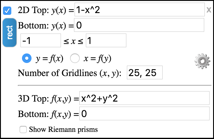
To add a region to the plot, select the option Region on the Add to graph drop-down menu. You'll see an object dialog appear like the following:
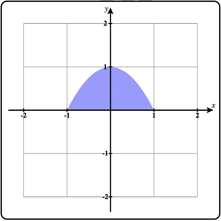
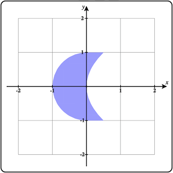
The 2D region in the \(xy\)-plane over which the region is defined is displayed in the 2D trace plot. See Figure 2.9.2.
This 2D region can be defined using two functions of \(x\) (top and bottom functions) and a range of \(x\)-values as shown above, or you can select \(x = f(y)\) and enter left and right functions of \(y\) and a range of \(y\)-values as shown below.
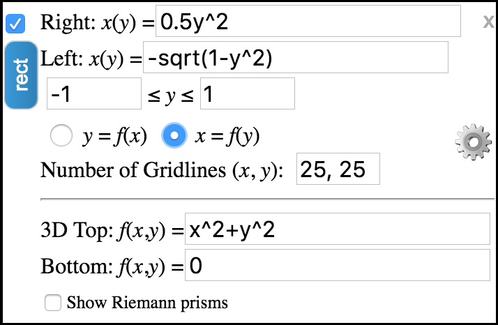
In either mode, you can adjust the number of gridlines in each direction from the default of 25 x 25.
To define the top and bottom surfaces for the region, enter the functions of \(x\) and \(y\) in the corresponding textboxes near the bottom of this dialog.
Now let's plot the default region. If not already set, select the option \(y = f(x)\text{.}\)

First clear the plot by clicking the clear plot button.
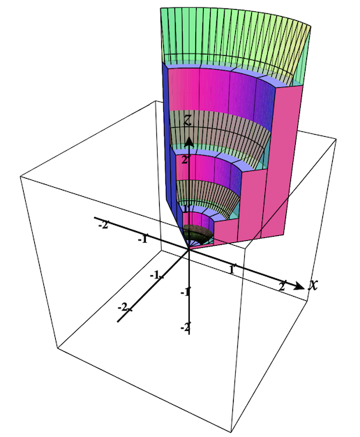
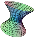
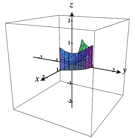
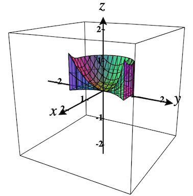
Then check the checkbox in the upper-left corner of this object to plot the default region. It should look like Figure 2.9.5 shown on the left. In Figure 2.9.6 you can see the default region for the \(x = f(y)\) option. Compare the graphs of the base region in the \(xy\)-planes above with the regions shown here.
Currently parameters are not yet supported in regions.
Subsection 2.9.1 Show Riemann Prisms
Select the checkbox labeled, Show Riemann Prisms. The region dialog should extend to show more options as shown in Figure 2.9.7 below. Note that if the region is already plotted, the prisms will automatically be added to the plot. Figure 2.9.8 shows the current region with prisms. It is zoomed in once as well, using the Zoom-in button.
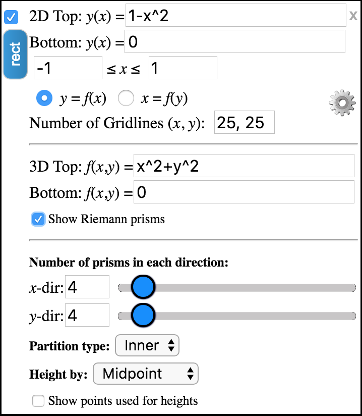
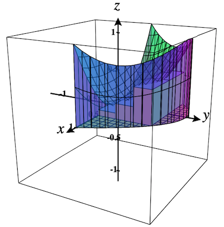
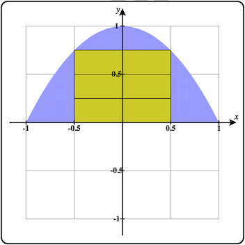
Figure 2.9.9 shows how the bases of the prisms are shown in the 2D plot as well.
The number of prisms in each direction specify the number that would be used for an outer partition. The default partition type is an inner partition that only uses the prisms whose bases are fully contained inside the 2D region.
You can vary the number of prisms to use in each direction using the textboxes or the sliders.
Partition type can be either Inner Partion (the default) or Outer Partition.
Height by specifies the point in the base of each prism that is to be used to determine the height of the prism on the surface. Options are: Midpoint, Upper-left, Upper-right, Lower-left, Lower-right.
Select Show points used for heights to see these points shown in the \(xy\)-plane and the points on the surfaces above/below shown as well.
Experiment with these options and see what each produces in the plot.
Subsection 2.9.2 Polar Regions
In addition to regions that use rectangular coordinates, CalcPlot3D also allows you to create regions in polar coordinates to help visualize double integrals in polar coordinates.
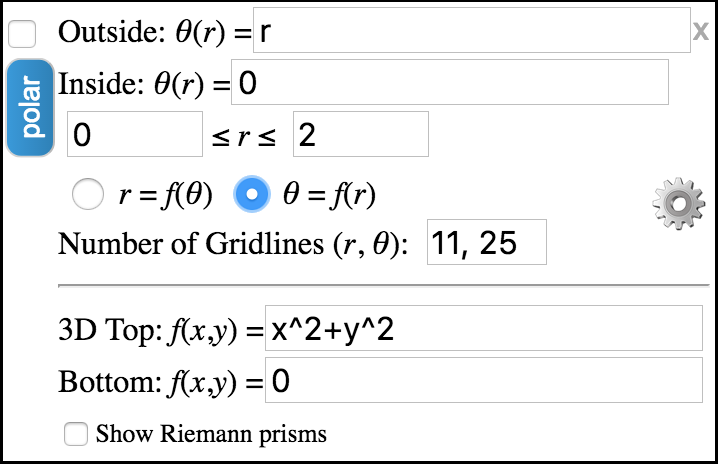
To switch to plot a polar region, click the sideways oriented button labeled, rect. It should change to read polar and the dialog and traceplane should change to appear as in Figure 2.9.10 and Figure 2.9.11.
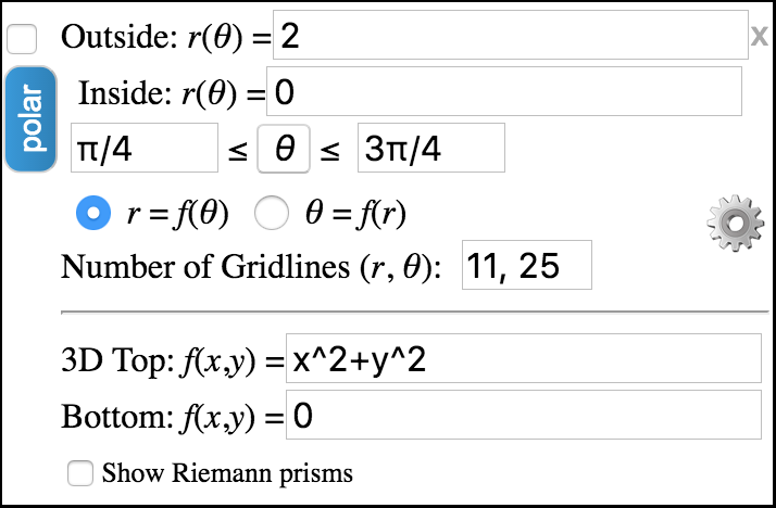
By default, the polar region is bounded by inside and outside functions of the form, \(r = f(\theta)\text{,}\) and a range of values for \(\theta\text{.}\) To use \(\theta\) in your functions, you can either type theta or you can click on the θ button while you are editing the inside or outside functions.
Below you can see this region plotted in the 3D plot.
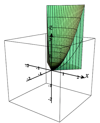
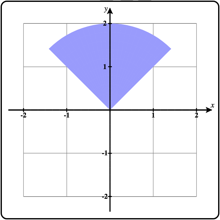
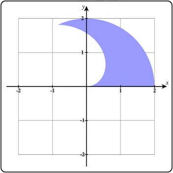
You can change the boundaries to be functions of the form, \(\theta = f(r)\) and specify a range for the values of \(r\text{.}\) Below you can see how the region dialog changes and the corresponding 2D base region in the \(xy\)-plane and 3D region plot.
Play with these options and see what you get.
Subsection 2.9.3 Polar Prisms
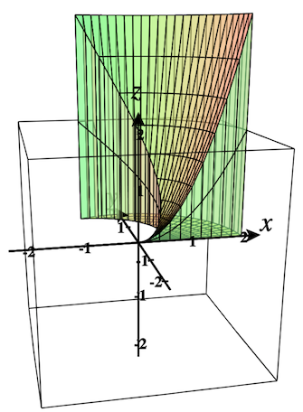
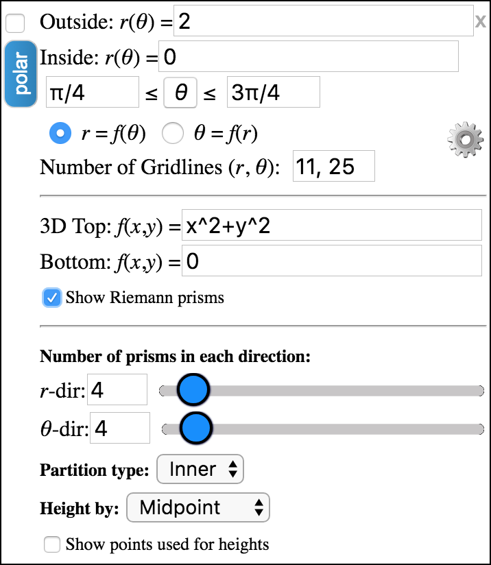
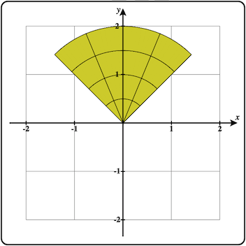
Just as we could plot the Riemann prisms above for regions in rectangular coordinates, we can plot the polar prisms that are relevant here. As above, just select the option to Show Riemann Prisms. The dialog will extend as before giving you the same options. See Figure 2.9.16. The only difference is that the bases of the prisms are not rectangles in the normal sense. They are “polar rectangles” instead. See the bases of the prisms in Figure 2.9.17.
The 3D polar region with polar prisms is shown below.